In-depth example of using HeartCV
Here we provide a detailed example of using HeartCV and explain each step of the workflow in depth.
The following imports are necessary for this example:
In [1]: import heartcv as hcv

In [2]: import matplotlib.pyplot as plt

In [3]: import cv2

In [4]: import numpy as np

In [5]: import vuba

In [6]: import pandas as pd
For this example, we will use video specifically for the freshwater pond snail, Radix balthica:
In [7]: video = hcv.load_example_video()
This returns a vuba.Video instance which we can read frames from like so:
# Grayscale frames are required for HeartCV
In [8]: frames = video.read(0, len(video), grayscale=True)
For a thorough overview of the capabilities of vuba, please refer to the corresponding documentation.
The first step of HeartCV involves the computation of a mean pixel value blockwise grid for the video provided:
In [9]: mpx = hcv.mpx_grid(frames, binsize=2)
Here we are downsampling each frame in the video by a factor of 2, i.e. 2 x 2 blocks of pixels are averaged. We can change this binning factor to as little or as much as we want - this will largely be dependent on what resolution you require and/or the speed you need for your application, respectively.
Once we’ve computed our mean pixel value grid for our video, we can compute the energy proxy traits present within the footage. Energy proxy traits (EPTs) are essentially power spectra derived from mean pixel value time-series present within video of live biological material. They are a holistic measure of the observable phenotype that animals exhibit (see Tills et al., 2021). However, here we are using EPTs for a different purpose: localising regions of cardiac activity. Because mean pixel value time-series of cardiac regions are quasi-periodic, they can be detected at specific frequency bands when such time-series are transformed to the frequency domain. To compute EPTs from the mean pixel value grid above we can use the following:
In [10]: ept = hcv.epts(mpx, video.fps)
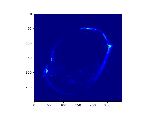
The output of heartcv.epts is two numpy arrays corresponding to the frequency and power outputs from performing welch’s method at each mean pixel value block. If we collapse these arrays to yield the total energy at each block, we get a heatmap coloured by the relative energy present within a block at all frequency bands:
# Frequency range
In [11]: freq, power = ept

In [12]: frequencies = freq[..., 0, 0]

In [13]: fmin, fmax = frequencies.min(), frequencies.max()

In [14]: print(fmin, fmax)
0.0 15.0

In [15]: heatmap = hcv.spectral_map(ept, frequencies=(fmin, fmax))

In [16]: plt.imshow(heatmap, cmap='jet')
Out[16]: <matplotlib.image.AxesImage at 0x7f5a106ee610>
However, for most instances we would not want information from all frequency bands since cardiac activity is likely to only be reflected at specific frequencies. Consequently, we can use a bandpass filter to attenuate frequencies at which we would not ordinarily expect cardiac activity for the animal at hand like so:
# 2-6 Hz is generally where most cardiac activity can be observed in hippo stage Radix balthica
In [17]: heatmap = hcv.spectral_map(ept, frequencies=(2, 6))

In [18]: plt.imshow(heatmap, cmap='jet')
Out[18]: <matplotlib.image.AxesImage at 0x7f5a106b15d0>
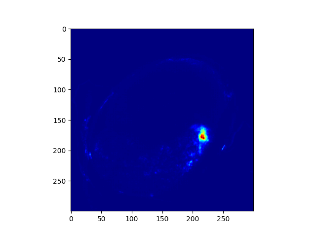
Now that we’ve performed this bandpass filter, we find that we actually have only a single bright spot in the heatmap, corresponding to the heart. Because these heatmaps are at a resolution smaller than the original video, we need to resize them so that we can segment to the desired regions:
In [19]: heatmap = cv2.resize(heatmap, video.resolution)
With our heatmap at the appropriate resolution, we can now perform segmentation via OTSU thresholding and contour filtering operations:
In [20]: roi = hcv.detect_largest(heatmap)
This gives a polygon that is fit to the largest shape detected by OTSU thresholding, which in this case is the heart. However, for most applications it is preferable to segment to a bounding box. To convert this polygon to a bounding box we can simply do the following:
In [21]: rectangle = vuba.fit_rectangles(roi, rotate=True)

In [22]: contour = cv2.boxPoints(rectangle)

In [23]: contour = np.int0(contour)

In [24]: first_frame = vuba.bgr(vuba.take_first(frames))

In [25]: vuba.draw_contours(first_frame, contour, -1, (0,255,0), 1)

In [26]: plt.imshow(first_frame, cmap='jet')
Out[26]: <matplotlib.image.AxesImage at 0x7f5a105d4d50>
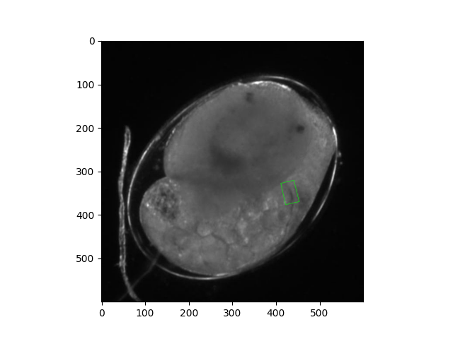
Note that here we specified that the bounding box fit should be by minimum area, and thus will be rotated (rotate=True). This generally results in much better segmentation to the region of interest as most applications will not have the heart perfectly oriented.
Now we can perform segmentation to this region using the following:
In [27]: at_roi = np.asarray(list(hcv.segment(frames, contour)))
We can validate that this is indeed the heart using an orthogonal view of the segmented frames:
# Taken from: https://stackoverflow.com/questions/11627362/how-to-straighten-a-rotated-rectangle-area-of-an-image-using-opencv-in-python/48553593#48553593
In [28]: def get_sub_image(img, rect):
   ....:     center, size, theta = rect
   ....:     center, size = tuple(map(int, center)), tuple(map(int, size))
   ....:     M = cv2.getRotationMatrix2D( center, theta, 1)
   ....:     dst = cv2.warpAffine(img, M, img.shape[:2])
   ....:     out = cv2.getRectSubPix(dst, size, center)
   ....:     return out
   ....:

In [29]: at_roi_sub = np.asarray([get_sub_image(frame, rectangle) for frame in frames])

In [30]: length, x, y = at_roi_sub.shape

In [31]: ix,iy = x // 2, y // 2

In [32]: x = at_roi_sub[:, ix, :]

In [33]: y = at_roi_sub[:, :, iy]

In [34]: fig, (ax1, ax2) = plt.subplots(2, 1)

In [35]: ax1.imshow(x.T, cmap='gray')
Out[35]: <matplotlib.image.AxesImage at 0x7f5a10517850>

In [36]: ax1.set_title('Horizontal view')
Out[36]: Text(0.5, 1.0, 'Horizontal view')

In [37]: ax2.imshow(y.T, cmap='gray')
Out[37]: <matplotlib.image.AxesImage at 0x7f5a104d40d0>

In [38]: ax2.set_title('Vertical view')
Out[38]: Text(0.5, 1.0, 'Vertical view')

In [39]: plt.draw()
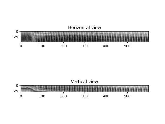
As we can see there is a clear rhythmic signal in the data, very similar to the m-modes one finds from videos of hearts obtained through other techniques (e.g. Fink et al., 2009).
Now that we’ve localised the cardiac region, the next step is to extract a signal that enables us to quantify when heart beats occur. In HeartCV, we do this by collapsing the segmented images above to a one dimensional vector by averaging each segmented frame, creating a mean pixel value time-series:
In [40]: v = at_roi.mean(axis=(1, 2))

In [41]: time = np.asarray([i/video.fps for i in range(len(v))])

In [42]: plt.plot(time, v, 'k')
Out[42]: [<matplotlib.lines.Line2D at 0x7f5a104aba50>]

In [43]: plt.xlabel('Time (seconds)')
Out[43]: Text(0.5, 0, 'Time (seconds)')

In [44]: plt.ylabel('Mean pixel value (px)')
Out[44]: Text(0, 0.5, 'Mean pixel value (px)')

In [45]: plt.draw()
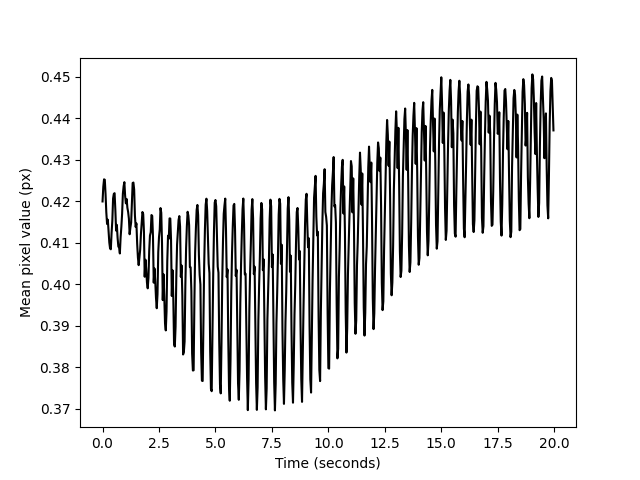
Because this signal is oscillatory in nature, we can leverage a multitude of peak detection methods to retrieve the peaks that correspond to a heart beat. We’ve found that automatic multiscale peak detection (AMPD) to perform particularly well on such data and so it is the one we provide with HeartCV:
In [46]: v = np.interp([i/3 for i in range(len(v)*3)], np.arange(0, len(v)), v) # upsample by a factor of 3 to improve peak detection

In [47]: peaks = hcv.find_peaks(v)

In [48]: time = np.asarray([i/(video.fps*3) for i in range(len(v))])

In [49]: plt.plot(time, v, 'k')
Out[49]: [<matplotlib.lines.Line2D at 0x7f59fc10e450>]

In [50]: plt.plot(time[peaks], v[peaks], 'or')
Out[50]: [<matplotlib.lines.Line2D at 0x7f59fc10e990>]

In [51]: plt.xlabel('Time (seconds)')
Out[51]: Text(0.5, 0, 'Time (seconds)')

In [52]: plt.ylabel('Mean pixel value (px)')
Out[52]: Text(0, 0.5, 'Mean pixel value (px)')

In [53]: plt.draw()
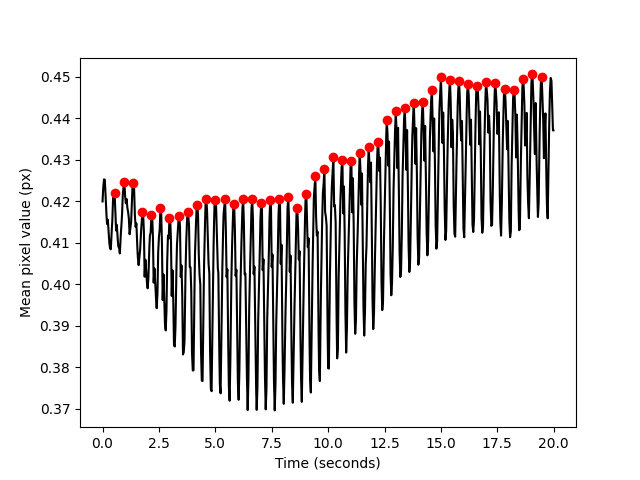
Note that we upsample the mean pixel value signal, this both improves peak detection performance but has also provided much more accurate results in comparison to manual quantification.
We can now use these peaks to compute various metrics of cardiac function as follows:
# Beat to beat intervals (seconds)
In [54]: hcv.b2b_intervals(peaks, video.fps*3)
Out[54]:
array([0.43333333, 0.4       , 0.4       , 0.4       , 0.4       ,
       0.4       , 0.43333333, 0.36666667, 0.43333333, 0.4       ,
       0.4       , 0.43333333, 0.4       , 0.4       , 0.4       ,
       0.4       , 0.4       , 0.4       , 0.4       , 0.4       ,
       0.4       , 0.4       , 0.4       , 0.4       , 0.4       ,
       0.36666667, 0.4       , 0.4       , 0.4       , 0.4       ,
       0.4       , 0.4       , 0.4       , 0.4       , 0.4       ,
       0.4       , 0.4       , 0.4       , 0.4       , 0.4       ,
       0.4       , 0.4       , 0.43333333, 0.4       , 0.4       ,
       0.4       , 0.43333333])

# Various cardiac statistics
In [55]: hcv.stats(peaks, len(video)*3, video.fps*3)
Out[55]:
{'bpm': 144.0,
 'min_b2b': 0.36666666666666664,
 'mean_b2b': 0.402836879432624,
 'median_b2b': 0.4,
 'max_b2b': 0.43333333333333335,
 'sd_b2b': 0.013456500681567575,
 'range_b2b': 0.06666666666666671,
 'rmssd': 0.020851441405707487}
Exporting such statistics can be done easily using pandas like so:
In [56]: data = hcv.stats(peaks, len(video)*3, video.fps*3)

# Convert data stats to list format for pandas below:
In [57]: for key, value in data.items():
   ....:         data[key] = [value]
   ....:

In [58]: df = pd.DataFrame(data=data)

In [59]: df.to_csv('./output.csv')